Analytic Beams
The analytic beams defined in pyuvdata are based on a base class,
pyuvdata.analytic_beam.AnalyticBeam, which ensures a standard interface
and can be used to define other analytic beams in a consistent way.
Evaluating analytic beams
To evaluate an analytic beam at one or more frequencies and in in one or more
directions, use either the pyuvdata.analytic_beam.AnalyticBeam.efield_eval()
or pyuvdata.analytic_beam.AnalyticBeam.power_eval() methods as appropriate.
Evaluating an Airy Beam power response
This code evaluates an Airy beam power response. Note that we exclude the cross
polarizations, since this is an unpolarized beam, the cross polarizations
are identical to the auto polarization power beams. If the cross polarizations
are included, the array returned from the power_eval method will be complex.
import numpy as np

from pyuvdata import AiryBeam

# Create an AiryBeam with a diameter of 14.5 meters
airy_beam = AiryBeam(diameter=14.5, include_cross_pols=False)

# set up zenith angle, azimuth and frequency arrays to evaluate with
az_grid = np.deg2rad(np.arange(0, 360))
za_grid = np.deg2rad(np.arange(0, 91))
az_array, za_array = np.meshgrid(az_grid, za_grid)

az_array = az_array.flatten()
za_array = za_array.flatten()

Nfreqs = 11
freqs = np.linspace(100, 200, 11) * 1e6

beam_vals = airy_beam.power_eval(
    az_array=az_array, za_array=za_array, freq_array=freqs
)
assert beam_vals.shape == (1, 2, 11, 91 * 360)
assert beam_vals.dtype == np.float64
Evaluating a Short Dipole Beam E-Field response
This code evaluates and plots a short (Herzian) dipole beam E-field response (also called the Jones matrix). Since it is the E-Field response, we have 4 effective maps because we have the response to each polarization basis vector for each feed. In the case of a short dipole, these maps do not have an imaginary part, but in general E-Field beams can be complex, so a complex array is returned.
import matplotlib.pyplot as plt
import numpy as np

from pyuvdata import ShortDipoleBeam

# Create an ShortDipoleBeam
dipole_beam = ShortDipoleBeam()

# set up zenith angle, azimuth and frequency arrays to evaluate with
az_grid = np.deg2rad(np.arange(0, 360))
za_grid = np.deg2rad(np.arange(0, 91))
az_array, za_array = np.meshgrid(az_grid, za_grid)

az_array = az_array.flatten()
za_array = za_array.flatten()

Nfreqs = 11
freqs = np.linspace(100, 200, 11) * 1e6

beam_vals = dipole_beam.efield_eval(
    az_array=az_array, za_array=za_array, freq_array=freqs
)
assert beam_vals.shape == (2, 2, 11, 91 * 360)
assert beam_vals.dtype == np.complex128
Plotting analytic beams
Plotting beams can be extremely helpful to reason about their behavior and whether they are implemented properly given the various conventions. To aid with this, a basic plotting method is available on AnalyticBeams.
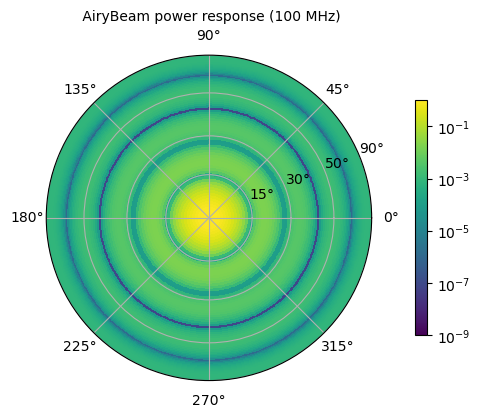
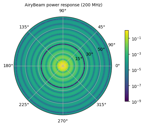
Plotting an Airy Beam power response
For unpolarized analytic beams, only a single feed is plotted (because all feeds are the same). Airy beams are frequency dependent, so we plot two frequencies to allow comparison.
from pyuvdata import AiryBeam

# Create an AiryBeam with a diameter of 14.5 meters with just one feed
airy_beam = AiryBeam(diameter=14.5, feed_array=["x"], include_cross_pols=False)

airy_beam.plot(
    beam_type="power",
    freq=100e6,
    logcolor=True,
    norm_kwargs={"vmin": 1e-9},
    savefile="Images/airy_beam_100MHz.png",
)
airy_beam.plot(
    beam_type="power",
    freq=200e6,
    logcolor=True,
    norm_kwargs={"vmin": 1e-9},
    savefile="Images/airy_beam_200MHz.png",
)
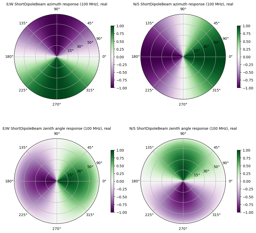
Plotting a Short Dipole Beam E-Field response
Polarized E-field beams are more complex because they represent the response from each feed to the 2 orthogonal directions on the sky. Looking at them carefully though allows us to check that everything is set up properly.
We use the following figure to illustrate the conventions. The two orthogonal polarization directions on the sky for analytic beams in pyuvdata are zenith angle, with is zero at zenith and decreasing towards the horizon and azimuth, which is zero at East and runs towards North, counter-clockwise as viewed from above. Note that this is consistent with the coordinate system of many EM beam simulators but different than the coordinate systems used in many radio astronomy contexts. The zenith angle polarization direction is shown in pink in the figure below and the azimuth angle polarization direction is shown in orange. We choose two locations, noted in green and blue, just off of zenith to the East and North to check the sign of the expected response for each feed. The expected signs are shown in the table below the figure.
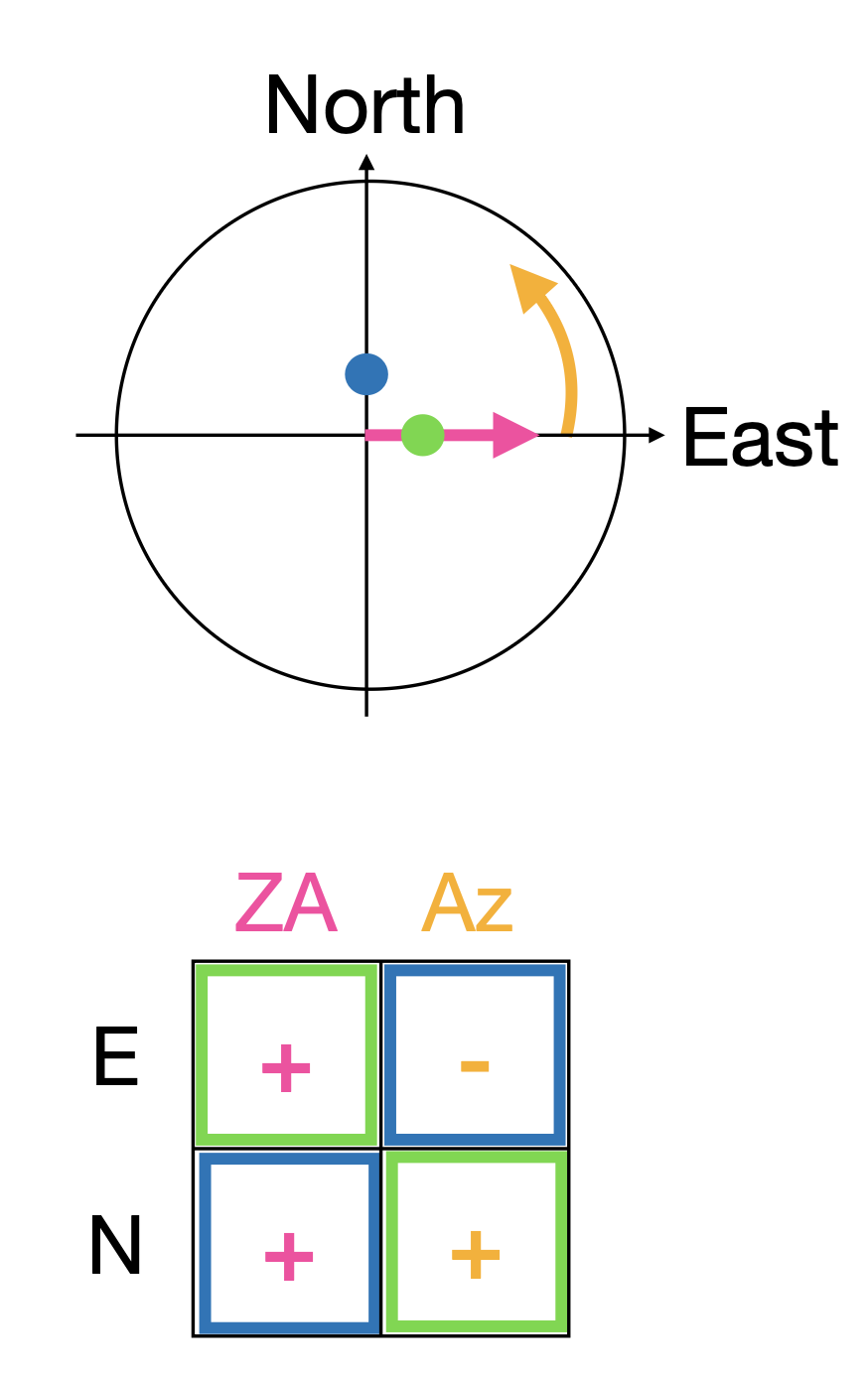
So the east dipole is expected to have a positive response to the zenith-angle aligned polarization just off of zenith in the East direction and a negative response to the azimuthal aligned polarization just of zenith in the North direction, which matches what we see in the following plots. Below we plot the real part for each feed and polarization orientation.
We can also check that the zenith-angle aligned polarization response goes to zero near the horizon for both feeds while the azimuthal aligned polarization response does not.
from pyuvdata import ShortDipoleBeam

# Create an ShortDipoleBeam
dipole_beam = ShortDipoleBeam()

dipole_beam.plot(beam_type="efield", freq=100e6, savefile="Images/short_dipole_beam.png")
Defining new analytic beams
We have worked to make defining new analytic beams as straight forward as possible.
The new beam needs to inherit from either the pyuvdata.analytic_beam.AnalyticBeam,
or the pyuvdata.analytic_beam.UnpolarizedAnalyticBeam, which are base
classes that specify what needs to be defined on the new class. Unpolarized
beams (based on the UnpolarizedAnalyticBeam class) have fewer things that
need to be specified.
Note that while unpolarized beams are simpler to define and think about, they are quite unphysical and can have results that may be surprising to radio astronomers. Since unpolarized feeds respond equally to all orientations of the E-field, if two feeds are specified they will have cross-feed power responses that are more similar to typical auto-feed power responses (and they will be identical to auto-feed power responses if the two feeds have the same beam shapes).
Setting parameters on the beam
If the new beam has any parameters that control the beam response (e.g. diameter),
The class must have an @dataclass decorator and the parameters must be listed
in the class definitions with type annotations and optionally defaults (these
are called fields in the dataclass, see the examples below and
dataclass for more details).
If you need to do some manipulation or validation of the parameters after they
are specified by the user, you can use the validate method to do that
(under the hood the validate method is called by the base object’s dataclass
__post_init__ method, so the validate method will always be called
when the class is instantiated).
The gaussian beam example below shows how this can be done.
Polarized beams
For polarized beams (based on the AnalyticBeam class), the following items
may be specified, the defaults on the AnalyticBeam class are noted:
feed_array: This an array of feed strings (a list can also be passed, it will be converted to an array). The default is["x", "y"]. This is a a dataclass field, so if it is specified, the class must have@dataclassdecorator and it should be specified with type annotations and optionally a default (see examples below).
x_orientation: For linear polarization feeds, this specifies what thexfeed polarization correspond to, allowed values are"east"or"north", the default is"east". Should be set toNonefor circularly polarized feeds. This is a a dataclass field, so if it is specified, the class must have@dataclassdecorator and it should be specified with type annotations and optionally a default (see examples below).
basis_vector_type: This defines the coordinate system for the polarization basis vectors, the default is"az_za". Currently only"az_za"is supported, which specifies that there are 2 vector directions (i.e.Naxes_vecis 2). This should be defined as a class variable (see examples below).
Defining the beam response
At least one of the _efield_eval or _power_eval methods must be
defined to specify the response of the new beam. Defining _efield_eval is
the most general approach because it can represent complex and negative going
E-field beams (if only _efield_eval defined, power beams will be calculated
from the E-field beams). If only _power_eval is defined, the E-field beam is
defined as the square root of the auto polarization power beam, so the E-field
beam will be real and positive definite. Both methods can be specified, which
may allow for computational efficiencies in some cases.
The inputs to the _efield_eval and _power_eval methods are the same and
give the directions (azimuth and zenith angle) and frequencies to evaluate the
beam. All three inputs must be two-dimensional with the first axis having the
length of the number of frequencies and the second axis having the having the
length of the number of directions (these are essentially the output of an
np.meshgrid on the direction and frequency vectors). The inputs are:
az_grid: an array of azimuthal values in radians for the directions to evaluate the beam. Shape: (number of frequencies, number of directions)
za_array: an array of zenith angle values in radians for the directions to evaluate the beam. Shape: (number of frequencies, number of directions)
freq_array: an array of frequencies in Hz at which to evaluate the beam. Shape: (number of frequencies, number of directions)
The _efield_eval and _power_eval methods must return arrays with the beam
response. The shapes and types of the returned arrays are:
_efield_eval: a complex array of beam responses with shape: (
Naxes_vec,Nfeeds,freq_array.size,az_array.size).Naxes_vecis 2 for the"az_za"basis, andNfeedsis typically 2.
_power_eval: an array with shape: (1,Npols,freq_array.size,az_array.size).Npolsis equal to eitherNfeedssquared ifinclude_cross_polswas set to True (the default) when the beam was instantiated orNfeedsifinclude_cross_polswas set to False. The array should be real ifinclude_cross_polswas set to False and it can be complex ifinclude_cross_polswas set to True (it will be cast to complex when it is called via thepower_evalmethod on the base class).
Below we provide some examples of beams defined in pyuvdata to make this more concrete.
Example: Defining simple unpolarized beams
Airy beams are unpolarized but frequency dependent and require one parameter,
the dish diameter in meters. Since the Airy beam E-field response goes negative,
the _efield_eval method is specified in this beam. The definition in pyuvdata
for the AiryBeam object is:
@dataclass(kw_only=True, eq=False)
class AiryBeam(UnpolarizedAnalyticBeam):
    """
    A zenith pointed Airy beam.

    Airy beams are the diffraction pattern of a circular aperture, so represent
    an idealized dish. Requires a dish diameter in meters and is inherently
    chromatic and unpolarized.

    The unpolarized nature leads to some results that may be surprising to radio
    astronomers: if two feeds are specified they will have identical responses
    and the cross power beam between the two feeds will be identical to the
    power beam for a single feed.

    Attributes
    ----------
    diameter : float
        Dish diameter in meters.

    Parameters
    ----------
    diameter : float
        Dish diameter in meters.
    include_cross_pols : bool
        Option to include the cross polarized beams (e.g. xy and yx or en and ne) for
        the power beam.

    """

    diameter: float

    # Have to define this because an Airy E-field response can go negative,
    # so it cannot just be calculated from the sqrt of a power beam.
    def _efield_eval(
        self, *, az_grid: FloatArray, za_grid: FloatArray, f_grid: FloatArray
    ) -> FloatArray:
        """Evaluate the efield at the given coordinates."""
        data_array = self._get_empty_data_array(az_grid.shape)

        kvals = (2.0 * np.pi) * f_grid / speed_of_light.to("m/s").value
        xvals = (self.diameter / 2.0) * np.sin(za_grid) * kvals
        values = np.zeros_like(xvals)
        nz = xvals != 0.0
        ze = xvals == 0.0
        values[nz] = 2.0 * j1(xvals[nz]) / xvals[nz]
        values[ze] = 1.0

        for fn in np.arange(self.Nfeeds):
            data_array[0, fn, :, :] = values / np.sqrt(2.0)
            data_array[1, fn, :, :] = values / np.sqrt(2.0)

        return data_array
Below we show how to define a cosine shaped beam with a single width parameter,
which can be defined with just the _power_eval method.
from dataclasses import dataclass

import numpy as np
from pyuvdata.analytic_beam import UnpolarizedAnalyticBeam
from pyuvdata.utils.types import FloatArray

@dataclass(kw_only=True)
class CosBeam(UnpolarizedAnalyticBeam):
    """
    A variable-width zenith pointed cosine beam.

    Attributes
    ----------
    width : float
        Width parameter, E-field goes like a cosine of width * zenith angle,
        power goes like the same cosine squared.

    Parameters
    ----------
    width : float
        Width parameter, E-field goes like a cosine of width * zenith angle,
        power goes like the same cosine squared.
    include_cross_pols : bool
        Option to include the cross polarized beams (e.g. xy and yx or en and ne) for
        the power beam.

    """

    width: float

    def _power_eval(
        self,
        *,
        az_grid: FloatArray,
        za_grid: FloatArray,
        f_grid: FloatArray,
    ) -> FloatArray:
        """Evaluate the power at the given coordinates."""

        data_array = self._get_empty_data_array(az_grid.shape, beam_type="power")

        for pol_i in np.arange(self.Npols):
            data_array[0, pol_i, :, :] = np.cos(self.width * za_grid) ** 2

        return data_array
Defining a cosine beam with no free parameters is even simpler:
import numpy as np
from pyuvdata.analytic_beam import UnpolarizedAnalyticBeam
from pyuvdata.utils.types import FloatArray

class CosBeam(UnpolarizedAnalyticBeam):
    """
    A zenith pointed cosine beam.

    Parameters
    ----------
    include_cross_pols : bool
        Option to include the cross polarized beams (e.g. xy and yx or en and ne) for
        the power beam.

    """

    def _power_eval(
        self,
        *,
        az_grid: FloatArray,
        za_grid: FloatArray,
        f_grid: FloatArray,
    ) -> FloatArray:
        """Evaluate the power at the given coordinates."""

        data_array = self._get_empty_data_array(az_grid.shape, beam_type="power")

        for pol_i in np.arange(self.Npols):
            data_array[0, pol_i, :, :] = np.cos(za_grid) ** 2

        return data_array
Example: Defining a beam with post init validation
The gaussian beam defined in pyuvdata is an unpolarized beam that has several
optional configurations that require some validation, which we do using the
validate method.
Here is the definition in pyuvdata for the GaussianBeam object and the
diameter_to_sigma function it uses:
def diameter_to_sigma(diameter: float, freq_array: FloatArray) -> float:
    """
    Find the sigma that gives a beam width similar to an Airy disk.

    Find the stddev of a gaussian with fwhm equal to that of
    an Airy disk's main lobe for a given diameter.

    Parameters
    ----------
    diameter : float
        Antenna diameter in meters
    freq_array : array of float
        Frequencies in Hz

    Returns
    -------
    sigma : float
        The standard deviation in zenith angle radians for a Gaussian beam
        with FWHM equal to that of an Airy disk's main lobe for an aperture
        with the given diameter.

    """
    wavelengths = speed_of_light.to("m/s").value / freq_array

    scalar = 2.2150894  # Found by fitting a Gaussian to an Airy disk function

    sigma = np.arcsin(scalar * wavelengths / (np.pi * diameter)) * 2 / 2.355

    return sigma
@dataclass(kw_only=True, eq=False)
class GaussianBeam(UnpolarizedAnalyticBeam):
    """
    A circular, zenith pointed Gaussian beam.

    Requires either a dish diameter in meters or a standard deviation sigma in
    radians. Gaussian beams specified by a diameter will have their width
    matched to an Airy beam at each simulated frequency, so are inherently
    chromatic. For Gaussian beams specified with sigma, the sigma_type defines
    whether the width specified by sigma specifies the width of the E-Field beam
    (default) or power beam in zenith angle. If only sigma is specified, the
    beam is achromatic, optionally both the spectral_index and reference_frequency
    parameters can be set to generate a chromatic beam with standard deviation
    defined by a power law:

    stddev(f) = sigma * (f/ref_freq)**(spectral_index)

    The unpolarized nature leads to some results that may be
    surprising to radio astronomers: if two feeds are specified they will have
    identical responses and the cross power beam between the two feeds will be
    identical to the power beam for a single feed.

    Attributes
    ----------
    sigma : float
        Standard deviation in radians for the gaussian beam. Only one of sigma
        and diameter should be set.
    sigma_type : str
        Either "efield" or "power" to indicate whether the sigma specifies the size of
        the efield or power beam. Ignored if `sigma` is None.
    diameter : float
        Dish diameter in meters to use to define the size of the gaussian beam, by
        matching the FWHM of the gaussian to the FWHM of an Airy disk. This will result
        in a frequency dependent beam.  Only one of sigma and diameter should be set.
    spectral_index : float
        Option to scale the gaussian beam width as a power law with frequency. If set
        to anything other than zero, the beam will be frequency dependent and the
        `reference_frequency` must be set. Ignored if `sigma` is None.
    reference_frequency : float
        The reference frequency for the beam width power law, required if `sigma` is not
        None and `spectral_index` is not zero. Ignored if `sigma` is None.

    Parameters
    ----------
    sigma : float
        Standard deviation in radians for the gaussian beam. Only one of sigma
        and diameter should be set.
    sigma_type : str
        Either "efield" or "power" to indicate whether the sigma specifies the size of
        the efield or power beam. Ignored if `sigma` is None.
    diameter : float
        Dish diameter in meters to use to define the size of the gaussian beam, by
        matching the FWHM of the gaussian to the FWHM of an Airy disk. This will result
        in a frequency dependent beam.  Only one of sigma and diameter should be set.
    spectral_index : float
        Option to scale the gaussian beam width as a power law with frequency. If set
        to anything other than zero, the beam will be frequency dependent and the
        `reference_frequency` must be set. Ignored if `sigma` is None.
    reference_frequency : float
        The reference frequency for the beam width power law, required if `sigma` is not
        None and `spectral_index` is not zero. Ignored if `sigma` is None.
    include_cross_pols : bool
        Option to include the cross polarized beams (e.g. xy and yx or en and ne) for
        the power beam.

    """

    sigma: float | None = None
    sigma_type: Literal["efield", "power"] = "efield"
    diameter: float | None = None
    spectral_index: float = 0.0
    reference_frequency: float = None

    def validate(self):
        """Post-initialization validation and conversions."""
        if (self.diameter is None and self.sigma is None) or (
            self.diameter is not None and self.sigma is not None
        ):
            if self.diameter is None:
                raise ValueError("Either diameter or sigma must be set.")
            else:
                raise ValueError("Only one of diameter or sigma can be set.")

        if self.sigma is not None:
            if self.sigma_type not in ["efield", "power"]:
                raise ValueError("sigma_type must be 'efield' or 'power'.")

            if self.sigma_type == "power":
                self.sigma = np.sqrt(2) * self.sigma

            if self.spectral_index != 0.0 and self.reference_frequency is None:
                raise ValueError(
                    "reference_frequency must be set if `spectral_index` is not zero."
                )
            if self.reference_frequency is None:
                self.reference_frequency = 1.0

    def get_sigmas(self, freq_array: FloatArray) -> FloatArray:
        """
        Get the sigmas for the gaussian beam using the diameter (if defined).

        Parameters
        ----------
        freq_array : array of floats
            Frequency values to get the sigmas for in Hertz.

        Returns
        -------
        sigmas : array_like of float
            Beam sigma values as a function of frequency. Size will match the
            freq_array size.

        """
        if self.diameter is not None:
            sigmas = diameter_to_sigma(self.diameter, freq_array)
        elif self.sigma is not None:
            sigmas = (
                self.sigma
                * (freq_array / self.reference_frequency) ** self.spectral_index
            )
        return sigmas

    def _power_eval(
        self, *, az_grid: FloatArray, za_grid: FloatArray, f_grid: FloatArray
    ) -> FloatArray:
        """Evaluate the power at the given coordinates."""
        sigmas = self.get_sigmas(f_grid)

        values = np.exp(-(za_grid**2) / (sigmas**2))
        data_array = self._get_empty_data_array(az_grid.shape, beam_type="power")
        for fn in np.arange(self.Npols):
            # For power beams the first axis is shallow because we don't have to worry
            # about polarization.
            data_array[0, fn, :, :] = values

        return data_array
Example: Defining a simple polarized beam
Short (Hertzian) dipole beams are polarized but frequency independent and do not
require any extra parameters. We just inherit the default values of feed_array
and x_orientation from the AnalyticBeam class, so do not list them here.
Note that we define both the _efield_eval and _power_eval methods because
we can use some trig identities to reduce the number of cos/sin evaluations for
the power calculation, but it would give the same results if the _power_eval
method was not defined (we have tests verifying this).
We handle the defaulting of the feed_array in the validate because dataclass
fields cannot have mutable defaults. We also do some other validation in that method.
The definition in pyuvdata for the ShortDipoleBeam object is:
class ShortDipoleBeam(AnalyticBeam):
    """
    A zenith pointed analytic short dipole beam with two crossed feeds.

    A classical short (Hertzian) dipole beam with two crossed feeds aligned east
    and north. Short dipole beams are intrinsically polarized but achromatic.
    Does not require any parameters, but the orientation of the dipole labelled
    as "x" can be specified to align "north" or "east" via the x_orientation
    parameter (matching the parameter of the same name on UVBeam and UVData
    objects).

    Attributes
    ----------
    feed_array : array-like of str
        Feeds to define this beam for, e.g. x & y.
    feed_angle : array-like of float
        Position angle of a given feed, units of radians. A feed angle of 0 is
        typically oriented toward zenith for steerable antennas, otherwise toward
        north for fixed antennas (e.g., HERA, LWA). More details on this can be found
        on the "Conventions" page of the docs.
    mount_type : str
        Antenna mount type, which describes the optics of the antenna in question.
        Supported options include: "alt-az" (primary rotates in azimuth and
        elevation), "equatorial" (primary rotates in hour angle and declination)
        "orbiting" (antenna is in motion, and its orientation depends on orbital
        parameters), "x-y" (primary rotates first in the plane connecting east,
        west, and zenith, and then perpendicular to that plane),
        "alt-az+nasmyth-r" ("alt-az" mount with a right-handed 90-degree tertiary
        mirror), "alt-az+nasmyth-l" ("alt-az" mount with a left-handed 90-degree
        tertiary mirror), "phased" (antenna is "electronically steered" by
        summing the voltages of multiple elements, e.g. MWA), "fixed" (antenna
        beam pattern is fixed in azimuth and elevation, e.g., HERA), and "other"
        (also referred to in some formats as "bizarre"). See the "Conventions"
        page of the documentation for further details.

    Parameters
    ----------
    feed_array : array-like of str
        Feeds to define this beam for, e.g. x & y or r & l. Default is ["x", "y"]
    feed_angle : array-like of float
        Position angle of a given feed, units of radians. A feed angle of 0 is
        typically oriented toward zenith for steerable antennas, otherwise toward
        north for fixed antennas (e.g., HERA, LWA). More details on this can be found
        on the "Conventions" page of the docs.
    mount_type : str
        Antenna mount type, which describes the optics of the antenna in question.
        Supported options include: "alt-az" (primary rotates in azimuth and
        elevation), "equatorial" (primary rotates in hour angle and declination)
        "orbiting" (antenna is in motion, and its orientation depends on orbital
        parameters), "x-y" (primary rotates first in the plane connecting east,
        west, and zenith, and then perpendicular to that plane),
        "alt-az+nasmyth-r" ("alt-az" mount with a right-handed 90-degree tertiary
        mirror), "alt-az+nasmyth-l" ("alt-az" mount with a left-handed 90-degree
        tertiary mirror), "phased" (antenna is "electronically steered" by
        summing the voltages of multiple elements, e.g. MWA), "fixed" (antenna
        beam pattern is fixed in azimuth and elevation, e.g., HERA), and "other"
        (also referred to in some formats as "bizarre"). See the "Conventions"
        page of the documentation for further details.
    include_cross_pols : bool
        Option to include the cross polarized beams (e.g. xy and yx or en and ne) for
        the power beam.
    x_orientation : str
        Physical orientation of the feed for the x feed. Not meaningful for
        unpolarized analytic beams, but clarifies the orientation of the dipole
        for for polarized beams like the ShortDipoleBeam and matches with the
        meaning on UVBeam objects. Used to set values of the feed_angle attribute,
        ignored in feed_angle is provided. Default is "east".

    """

    basis_vector_type = "az_za"

    def validate(self):
        """Post-initialization validation and conversions."""
        if self.feed_array is None:
            self.feed_array = ["x", "y"]
        self.feed_array = np.asarray(self.feed_array)

        allowed_feeds = ["n", "e", "x", "y"]
        for feed in self.feed_array:
            if feed not in allowed_feeds:
                raise ValueError(
                    f"Feeds must be one of: {allowed_feeds}, "
                    f"got feeds: {self.feed_array}"
                )

        if self.feed_angle is not None:
            x_orient = utils.pol.get_x_orientation_from_feeds(
                feed_array=self.feed_array, feed_angle=self.feed_angle, tols=[0, 1e-6]
            )
            if x_orient is None:
                raise NotImplementedError(
                    "ShortDipoleBeams currently only support dipoles aligned to East "
                    "and North, it does not yet have support for arbitrary feed angles."
                )
            else:
                # use the standard feed angles for consistency
                _, _, feed_angle = utils.pol.get_feeds_from_x_orientation(
                    x_orientation=x_orient,
                    nants=1,
                    feed_array=self.feed_array[np.newaxis, :],
                )
                self.feed_angle = np.squeeze(feed_angle)

    def _efield_eval(
        self, *, az_grid: FloatArray, za_grid: FloatArray, f_grid: FloatArray
    ) -> FloatArray:
        """Evaluate the efield at the given coordinates."""
        data_array = self._get_empty_data_array(az_grid.shape)

        # The first dimension is for [azimuth, zenith angle] in that order
        # the second dimension is for feed [e, n] in that order
        data_array[0, self.east_ind] = -np.sin(az_grid)
        data_array[0, self.north_ind] = np.cos(az_grid)
        data_array[1, self.east_ind] = np.cos(za_grid) * np.cos(az_grid)
        data_array[1, self.north_ind] = np.cos(za_grid) * np.sin(az_grid)

        return data_array

    def _power_eval(
        self, *, az_grid: FloatArray, za_grid: FloatArray, f_grid: FloatArray
    ) -> FloatArray:
        """Evaluate the power at the given coordinates."""
        data_array = self._get_empty_data_array(az_grid.shape, beam_type="power")

        # these are just the sum in quadrature of the efield components.
        # some trig work is done to reduce the number of cos/sin evaluations
        data_array[0, 0] = 1 - (np.sin(za_grid) * np.cos(az_grid)) ** 2
        data_array[0, 1] = 1 - (np.sin(za_grid) * np.sin(az_grid)) ** 2

        if self.Npols > self.Nfeeds:
            # cross pols are included
            data_array[0, 2] = -(np.sin(za_grid) ** 2) * np.sin(2.0 * az_grid) / 2.0
            data_array[0, 3] = data_array[0, 2]

        return data_array