UVData

UVData objects hold all of the metadata and data required to analyze interferometric data sets. Interferometric data is fundamentally tied to baselines, which are composed of pairs of antennas. Visibilities, the measured quantity recorded from interferometers, are complex numbers per baseline, time, frequency and instrumental polarization. On UVData objects, visibilities are held in the data_array. The data_array has axes corresponding to baseline-time, frequency and instrumental polarization, so the baselines and times are indexed together. This is because it is not uncommon for interferometers not to record every baseline at every time for several reasons (including baseline-dependent averaging). Note that UVData can also support combining the frequency and polarization axis, which can be useful in certain circumstances, objects represented this way are called flex_pol objects and are more fully described in UVData: flex_pol objects.

Metadata that is associated with the telescope (as opposed to the data set) is stored in a pyuvdata.Telescope object as the telescope attribute on a UVData object. This includes metadata related to the telescope location, antenna names, numbers and positions as well as other telescope metadata. The antennas are described in two ways: with antenna numbers and antenna names. The antenna numbers should not be confused with indices – they are not required to start at zero or to be contiguous, although it is not uncommon for some telescopes to number them like indices. On UVData objects, the names and numbers are held in the telescope.antenna_names and telescope.antenna_numbers attributes respectively. These are arranged in the same order so that an antenna number can be used to identify an antenna name and vice versa. Note that not all the antennas listed in telescope.antenna_numbers and telescope.antenna_names are guaranteed to have visibilities associated with them in the data_array.

For most users, the convenience methods for quick data access (see UVData: Quick data access) are the easiest way to get data for particular sets of baselines. Those methods take the antenna numbers (i.e. numbers listed in telescope.antenna_numbers) as inputs. Users interested in indexing/manipulating the data array directly can find more information below.

The antenna numbers associated with each visibility are held in the ant_1_array and ant_2_array attributes. These arrays have the same length as the data_array along the baseline-time axis, and which array the numbers appear in (ant_1_array vs ant_2_array) indicates the direction of the baseline. On UVData objects, the baseline vector is defined to point from antenna 1 to antenna 2, so it is given by the position of antenna 2 minus the position of antenna 1. Since the ant_1_array and ant_2_array attributes have the length of the baseline-time axis, when there is more than one time integration in the data there are many repetitions of each baseline. The times for each visibility are given by the time_array attribute which also has the same length (the length of the baseline-time axis on the data_array).

There is also a baseline_array attribute with baseline numbers defined from the ant_1_array and ant_2_array as \(baseline = 2048 \times (antenna_1) + (antenna_2) + 2^{16}\). This gives a unique baseline number for each antenna pair and can be a useful way to identify visibilities associated with particular baselines. The baseline_array attribute has the same length as the ant_1_array and ant_2_array (the length of the baseline-time axis on the data_array).

Note

Our tutorial uses small data files for examples. The data files are hosted in the the RASG datasets repo, organized by data type and telescope. In the tutorials this data is downloaded and cached using the pooch package via the pyuvdata.datasets.fetch_data function. To run those commands you’ll need to have pooch installed (you can install it yourself or use pip install pyuvdata[tutorial]). Note that pooch will download the file the first time you ask for it and save it in a cache folder, subsequent calls to fetch that data will not re-download it.

UVData: Instantiating a UVData object from a file (i.e. reading data)

Use the pyuvdata.UVData.from_file() to instantiate a UVData object from data in a file (alternatively you can create an object with no inputs and then call the pyuvdata.UVData.read() method). Most file types require a single file or folder to instantiate an object, FHD and raw MWA correlator data sets require the user to specify multiple files for each dataset.

pyuvdata can also be used to create a UVData object from arrays in memory (see UVData: Instantiating from arrays in memory) and to read in multiple datasets (files) into a single object (see d) Reading multiple files.).

Note

Reading or writing CASA Measurement sets requires python-casacore to be installed (see the readme for details). Note that the python-casacore and casatools/casatasks packages are incompatible – importing them both causes segfaults. Reading or writing Miriad files is not supported on Windows.

a) Instantiate an object from a single file or folder

UVFITS and uvh5 and datasets are stored in a single file. Miriad, CASA Measurement Sets and MIR datasets are stored in structured folders, for these file types pass in the folder name.

from pyuvdata import UVData
from pyuvdata.datasets import fetch_data

filename = fetch_data("vla_casa_tutorial_uvfits")
uvd = UVData.from_file(filename)

b) Instantiate an object from an FHD dataset

When reading FHD datasets, we need to pass in several auxilliary files.

import os
from pyuvdata import UVData
from pyuvdata.datasets import fetch_data

# Set up the files we need
fhd_prefix = '1061316296_'
fhd_path = fetch_data("mwa_fhd")
fhd_vis_files = [os.path.join(fhd_path, "vis_data", fhd_prefix + f) for f in ["vis_XX.sav", "vis_YY.sav"]]
flags_file = os.path.join(fhd_path, "vis_data", fhd_prefix + "flags.sav")
layout_file = os.path.join(fhd_path, "metadata", fhd_prefix + "layout.sav")
params_file = os.path.join(fhd_path, "metadata", fhd_prefix + "params.sav")
settings_file = os.path.join(fhd_path, "metadata", fhd_prefix + "settings.txt")

uvd = UVData.from_file(
  fhd_vis_files,
  flags_file=flags_file,
  layout_file=layout_file,
  params_file=params_file,
  settings_file=settings_file,
)

c) Instantiate an object from a raw MWA correlator dataset

The MWA correlator writes FITS files containing the correlator dumps (but lacking metadata and not conforming to the uvfits format). pyuvdata can read these files from both the Legacy and MWAX correlator versions, along with MWA metafits files (containing the required metadata), into a UVData object. There are also options for applying cable length corrections, dividing out digital gains, dividing out the coarse band shape, common flagging patterns, using AOFlagger flag files, and phasing the data to the pointing center. It is also optional to apply a Van Vleck correction for Legacy correlator data. The default for this correction is to use a Chebyshev polynomial approximation, and there is an option to instead use a slower integral implementation.

from pyuvdata import UVData
from pyuvdata.datasets import fetch_data

# Construct the list of files. Separate files for each coarse band, the
# associated metafits file is also required.
filelist = fetch_data(["mwa_2015_metafits", "mwa_2015_raw_gpubox01"])

# Apply cable corrections and routine time/frequency flagging, phase data to pointing center
uvd = UVData().from_file(filelist, correct_cable_len=True, phase_to_pointing_center=True, flag_init=True)

c) Options for SMA MIR data sets

The SMA has its own bespoke file format known as MIR (no relation to MIRIAD), which most users prefer to convert to the CASA-based Measurement Sets (MS) for further processing. The pyuvdata.UVData.from_file() method (and by extension, pyuvdata.UVData.read() as well) has support for a few extra keywords that are specific to the MIR file format. These keywords fall broadly into two groups: selection, and visibility handling.

In addition to the selection keywords supported with UVData objects, there are a few extra keywords supported for MIR data sets: - corrchunk: Specifies (typically DSB) correlator window(s) to load.

• receiver: Specifies a receiver type (generally some combination of “230”, “240”,

  “345”, and/or “400”) to load, with different receivers typically used to target different bands and/or polarizations.

• sideband: Specifies which sideband to load, with the two options being “l” for

  lower and “u” for upper.

• pseudo_contSpecifies whether to load the “pseudo-continuum” data, which is

  constructed as the average of all channels across a single spectral window (set to False by default).

• select_whereAn keyword which allows for more advanced selection criterion.

  See the documentation in pyuvdata.mir_parser.MirParser() for more details.

Some example use cases for the selection keywords:

from pyuvdata import UVData
from pyuvdata.datasets import fetch_data

# Create a path to the SMA MIR test data set in pyuvdata
data_path = fetch_data("sma_mir")
# Let's first try loading just the "230" receivers.
uvd = UVData.from_file(data_path, receivers="230")
assert (uvd.Npols, uvd.Nfreqs) == (1, 131072)

# Now try one sideband, say the lower ("l")
uvd.read(data_path, sidebands="l")
assert (uvd.Npols, uvd.Nfreqs) == (2, 65536)

# Now try one just one chunk (2)
uvd.read(data_path, corrchunk=2)
assert (uvd.Npols, uvd.Nfreqs) == (2, 32768)

# Now all together -- "230" receiver, "l" sideband, chunks 1 and 3
uvd.read(data_path, receivers="230", sidebands="l", corrchunk=[1, 3])
assert (uvd.Npols, uvd.Nfreqs) == (1, 32768)

As for visibility handling keywords:

• rechunk: Number of channels to spectrally average the data over on read. This is

  generally the most commonly used keyword, as it reduces the memory/disk space needed to complete read/write operations.

• apply_tsys: Normalize the data using system temperature measurements to produces

  values in (uncalibrated) Jy (default is True).

• apply_flags: Apply on-line flags (default is True).

For example, the native resolution of the test MIR dataset is 140 kHz – to average this down by a factor of 64 (8.96 MHz resolution) do the following:

from pyuvdata import UVData
from pyuvdata.datasets import fetch_data

# Build a path to the test SMA data set
data_path = fetch_data("sma_mir")
# Set things up to average over 64-channel blocks.
uvd = UVData.from_file(data_path, rechunk=64)

Warning

Reading and writing of MIR data will on occasion generate a warning message about the LSTs not being correct. This warning is spurious, and a byproduct how LST values are calculated at time of write (polled average versus calculated based on the timestamp/integration midpoint), and can safely be ignored.

UVData: Writing UVData objects to disk

pyuvdata can write UVData objects to UVFITS, Miriad, CASA Measurement Set and uvh5 files. Each of these has an associated write method: pyuvdata.UVData.write_uvfits(), pyuvdata.UVData.write_miriad(), pyuvdata.UVData.write_ms(), pyuvdata.UVData.write_uvh5(), which only require a filename (or folder name for Miriad and CASA Measurement Sets) to write the data to.

pyuvdata can be used to simply convert data from one file type to another by reading in one file type and writing out another.

import os
from pyuvdata import UVData
from pyuvdata.datasets import fetch_data

ms_file = fetch_data("vla_casa_tutorial_ms")
# Instantiate an object from a measurement set
uvd = UVData.from_file(ms_file)

# Write the data out to a uvfits file
write_file = os.path.join(".", "tutorial.uvfits")
uvd.write_uvfits(write_file)

UVData: Quick data access

A small suite of functions are available to quickly access the underlying numpy arrays of data, flags, and nsamples. Although the user can perform this indexing by hand, several convenience functions exist to easily extract specific subsets corresponding to antenna-pair and/or polarization combinations. There are three specific methods that will return numpy arrays: pyuvdata.UVData.get_data(), pyuvdata.UVData.get_flags(), and pyuvdata.UVData.get_nsamples(). When possible, these methods will return numpy MemoryView objects, which is relatively fast and adds minimal memory overhead. There are also corresponding methods pyuvdata.UVData.set_data(), pyuvdata.UVData.set_flags(), and pyuvdata.UVData.set_nsamples() which will overwrite sections of these datasets with user-provided data.

a) Data for single antenna pair / polarization combination.

from pyuvdata import UVData
from pyuvdata.datasets import fetch_data

filename = fetch_data("vla_casa_tutorial_uvfits")
uvd = UVData.from_file(filename)
data = uvd.get_data(1, 2, "rr")  # data for ant1=1, ant2=2, pol="rr"
times = uvd.get_times(1, 2)  # times for ant1=1, ant2=2 (0th axis of "data" above)
assert data.shape == (9, 64)
assert times.shape == (9,)

# One can equivalently make any of these calls with the input wrapped in a tuple.
data = uvd.get_data((1, 2, "rr"))
times = uvd.get_times((1, 2))

b) Flags and nsamples for above data.

from pyuvdata import UVData
from pyuvdata.datasets import fetch_data

filename = fetch_data("vla_casa_tutorial_uvfits")
uvd = UVData.from_file(filename)

flags = uvd.get_flags(1, 2, "rr")
nsamples = uvd.get_nsamples(1, 2, "rr")
assert flags.shape == (9, 64)
assert nsamples.shape == (9, 64)

c) Data for single antenna pair, all polarizations.

from pyuvdata import UVData
from pyuvdata.datasets import fetch_data

filename = fetch_data("vla_casa_tutorial_uvfits")
uvd = UVData.from_file(filename)

data = uvd.get_data(1, 2)
assert data.shape == (9, 64, 4)

# Can also give baseline number, this gives the same array:
data2 = uvd.get_data(uvd.antnums_to_baseline(1, 2))

d) Data for single polarization, all baselines.

from pyuvdata import UVData
from pyuvdata.datasets import fetch_data

filename = fetch_data("vla_casa_tutorial_uvfits")
uvd = UVData.from_file(filename)

data = uvd.get_data("rr")
assert data.shape == (1360, 64)

e) Update data arrays in place for UVData

There are methods on UVData objects which allow for updating the data, flags, or nsamples arrays in place. We show how to use the pyuvdata.UVData.set_data() method below, and note there are analogous pyuvdata.UVData.set_flags() and pyuvdata.UVData.set_nsamples() methods.

from pyuvdata import UVData
from pyuvdata.datasets import fetch_data

filename = fetch_data("vla_casa_tutorial_uvfits")
uvd = UVData.from_file(filename)

data = uvd.get_data(1, 2, "rr", force_copy=True, squeeze="none")
data *= 2
uvd.set_data(data, 1, 2, "rr")

f) Iterate over all antenna pair / polarizations.

from pyuvdata import UVData
from pyuvdata.datasets import fetch_data

filename = fetch_data("vla_casa_tutorial_uvfits")
uvd = UVData.from_file(filename)

for key, data in uvd.antpairpol_iter():
    flags = uvd.get_flags(key)
    nsamples = uvd.get_nsamples(key)

  # Do something with the data, flags, nsamples

g) Convenience functions to ask what antennas, baselines, and pols are in the data.

from pyuvdata import UVData
from pyuvdata.datasets import fetch_data

filename = fetch_data("vla_casa_tutorial_uvfits")
uvd = UVData.from_file(filename)

# Get all unique antennas in data
unique_ants = uvd.get_ants()

# Get all baseline nums in data.
bl_nums = uvd.get_baseline_nums()

# Get all (ordered) antenna pairs in data (same info as baseline_nums)
antpairs = uvd.get_antpairs()

# Get all antenna pairs and polarizations, i.e. keys produced in UVData.antpairpol_iter()
antpair_pols = uvd.get_antpairpols()

h) Quick access to file attributes of a UV* object (UVData, UVCal, UVBeam)

## in bash ##
# Print data_array.shape to stdout
pyuvdata_inspect.py --attr=data_array.shape <uv*_file>

# Print Ntimes,Nfreqs,Nbls to stdout
pyuvdata_inspect.py --attr=Ntimes,Nfreqs,Nbls <uv*_file>

# Load object to instance name "uv" and will remain in interpreter
pyuvdata_inspect.py -i <uv*_file>

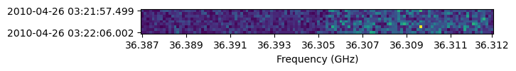
UVData: Plotting

Making a simple waterfall plot.

Note: there is now support for reading in only part of a file for many file types (see UVData: Working with large files), so you need not read in the entire file to plot one waterfall.

from astropy.time import Time
import numpy as np
import matplotlib.pyplot as plt
from pyuvdata import UVData
from pyuvdata.datasets import fetch_data

filename = fetch_data("vla_casa_tutorial_uvfits")
uvd = UVData.from_file(filename)

# get the data for a single baseline and polarization
waterfall_data = uvd.get_data((1, 2, uvd.polarization_array[0]))
# get the corresponding times for this waterfall
waterfall_times = Time(uvd.get_times((1, 2, uvd.polarization_array[0])), format="jd").iso

# Amplitude waterfall for all spectral channels and 0th polarization
fig, ax = plt.subplots(1, 1)
_ = ax.imshow(np.abs(waterfall_data), interpolation="none", origin="lower")
_ = ax.set_yticks([0, waterfall_times.size - 1])
_ = ax.set_yticklabels([waterfall_times[0], waterfall_times[1]])
freq_tick_inds = np.concatenate((np.arange(0, uvd.Nfreqs, 16), [uvd.Nfreqs-1]))
_ = ax.set_xticks(freq_tick_inds)
_ = ax.set_xticklabels([f"{val:.3f}" for val in uvd.freq_array[freq_tick_inds]*1e-9])
_ = ax.set_xlabel("Frequency (GHz)")

UVData: Selecting data

The pyuvdata.UVData.select() method lets you select specific antennas (by number or name), antenna pairs, frequencies (in Hz or by channel number), times (or time range), local sidereal time (LST) (or LST range), or polarizations to keep in the object while removing others. By default, pyuvdata.UVData.select() will select data that matches the supplied criteria, but by setting invert=True, you can instead deselect this data and preserve only that which does not match the selection.

Note: The same select interface is now supported on the read for many file types (see UVData: Working with large files), so you need not read in the entire file before doing the select.

a) Select 3 antennas to keep using the antenna number.

from pyuvdata import UVData
from pyuvdata.datasets import fetch_data

filename = fetch_data("vla_casa_tutorial_uvfits")
uvd = UVData.from_file(filename)
assert uvd.Nants_data == 18

uvd.select(antenna_nums=[1, 12, 21])
assert uvd.Nants_data == 3
assert uvd.get_ants().tolist() == [1, 12, 21]

b) Select 3 antennas by name and 4 frequencies to keep

from pyuvdata import UVData
from pyuvdata.datasets import fetch_data

filename = fetch_data("vla_casa_tutorial_uvfits")
uvd = UVData.from_file(filename)
assert uvd.Nants_data == 18
assert uvd.Nfreqs == 64

uvd.select(antenna_names=["N02", "E09", "W06"], frequencies=uvd.freq_array[0:4])
assert uvd.Nants_data == 3
assert uvd.Nfreqs == 4

c) Select a few antenna pairs to keep

from pyuvdata import UVData
from pyuvdata.datasets import fetch_data

filename = fetch_data("vla_casa_tutorial_uvfits")
uvd = UVData.from_file(filename)

# note that order of the values in the pair does not matter
uvd.select(bls=[(1, 2), (7, 1), (1, 21)])

# get all the antenna pairs after the select
antpairs = uvd.get_antpairs()
# note that the antpair is listed as it is in the data, not as it was selected on.
assert antpairs == [(1, 2), (1, 7), (1, 21)]

d) Select antenna pairs using baseline numbers

from pyuvdata import UVData
from pyuvdata.datasets import fetch_data

filename = fetch_data("vla_casa_tutorial_uvfits")
uvd = UVData.from_file(filename)

# select baselines using the baseline numbers
uvd.select(bls=[73736, 73753, 81945])
print(uvd.get_antpairs())
assert uvd.get_antpairs() == [(4, 8), (4, 25), (8, 25)]

e) Select polarizations

Selecting on polarizations can be done either using the polarization numbers or the polarization strings (e.g. “xx” or “yy” for linear polarizations or “rr” or “ll” for circular polarizations). Under special circumstances, where x-polarization feeds (as recorded in telescope.feed_array) are aligned to 0 or 90 degrees relative to a line perpendicular to the horizon (as record in telescope.feed_angle) and/or y-polarization are aligned to -90 or 0 degrees, strings representing the cardinal orientation of the dipole can also be used (e.g. “nn” or “ee”).

from pyuvdata import utils, UVData
from pyuvdata.datasets import fetch_data

filename = fetch_data("vla_casa_tutorial_uvfits")
uvd = UVData.from_file(filename)

# polarization numbers can be found in the polarization_array
assert uvd.polarization_array.tolist() == [-1, -2, -3, -4]

# polarization numbers can be converted to strings using a utility function
assert utils.polnum2str(uvd.polarization_array) == ['rr', 'll', 'rl', 'lr']

# select polarizations using the polarization numbers
uvd.select(polarizations=[-1, -2, -3])
assert uvd.polarization_array.tolist() == [-1, -2, -3]
assert utils.polnum2str(uvd.polarization_array) == ['rr', 'll', 'rl']

# select polarizations using the polarization strings
uvd.select(polarizations=["rr", "ll"])
assert uvd.polarization_array.tolist() == [-1, -2]
assert utils.polnum2str(uvd.polarization_array) == ['rr', 'll']

# Now deselect polarizations
uvd.select(polarizations=["ll"], invert=True)
assert uvd.polarization_array.tolist() == [-1]
assert utils.polnum2str(uvd.polarization_array) == ['rr']

# read in a file with linear polarizations and an x_orientation
filename = fetch_data("hera_h3c_uvh5")
uvd = UVData.from_file(filename)
assert uvd.polarization_array.tolist() == [-5, -6]
assert utils.polnum2str(uvd.polarization_array) == ['xx', 'yy']

# check x_orientation
assert uvd.telescope.get_x_orientation_from_feeds() == "north"

# select polarizations using the physical orientation strings
uvd.select(polarizations=["ee"])
assert uvd.polarization_array.tolist() == [-6]
assert utils.polnum2str(uvd.polarization_array) == ['yy']

f) Select antenna pairs and polarizations using ant_str argument

Basic options are “auto”, “cross”, or “all”. “auto” returns just the autocorrelations (all pols), while “cross” returns just the cross-correlations (all pols). The ant_str can also contain:

1. Individual antenna number(s):

• 1: returns all antenna pairs containing antenna number 1 (including the auto correlation)

• 1,2: returns all antenna pairs containing antennas 1 and/or 2

from pyuvdata import UVData
from pyuvdata.datasets import fetch_data

filename = fetch_data("vla_casa_tutorial_uvfits")
uvd = UVData.from_file(filename)

# check the number of baselines (antenna pairs) in the original file
assert uvd.Nbls == 153

# Apply select to UVData object
uvd.select(ant_str="1,2,3")

# check the number of baselines (antenna pairs) after the select
assert uvd.Nbls == 48

2. Individual baseline(s):

• 1_2: returns only the antenna pair (1,2)

• 1_2,1_3,1_10: returns antenna pairs (1,2),(1,3),(1,10)

• (1,2)_3: returns antenna pairs (1,3),(2,3)

• 1_(2,3): returns antenna pairs (1,2),(1,3)

from pyuvdata import UVData
from pyuvdata.datasets import fetch_data

filename = fetch_data("vla_casa_tutorial_uvfits")
uvd = UVData.from_file(filename)

# check the number of baselines (antenna pairs) in the original file
assert uvd.Nbls == 153

# Apply select to UVData object
uvd.select(ant_str="(1,2)_(3,7)")

# check the antenna pairs after the select
assert uvd.get_antpairs() == [(1, 3), (1, 7), (2, 3), (2, 7)]

3. Antenna number(s) and polarization(s):

When polarization information is passed with antenna numbers, all antenna pairs kept in the object will retain data for each specified polarization

• 1x: returns all antenna pairs containing antenna number 1 and polarizations xx and xy

• 2x_3y: returns the antenna pair (2,3) and polarization xy

• 1r_2l,1l_3l,1r_4r: returns antenna pairs (1,2), (1,3), (1,4) and polarizations rr, ll, and rl. This yields a complete list of baselines with polarizations of 1r_2l, 1l_2l, 1r_2r, 1r_3l, 1l_3l, 1r_3r, 1r_11l, 1l_11l, and 1r_11r.

• (1x,2y)_(3x,4y): returns antenna pairs (1,3),(1,4),(2,3),(2,4) and polarizations xx, yy, xy, and yx

• 2l_3: returns antenna pair (2,3) and polarizations ll and lr

• 2r_3: returns antenna pair (2,3) and polarizations rr and rl

• 1l_3,2x_3: returns antenna pairs (1,3), (2,3) and polarizations ll, lr, xx, and xy

• 1_3l,2_3x: returns antenna pairs (1,3), (2,3) and polarizations ll, rl, xx, and yx

from pyuvdata import UVData
from pyuvdata.datasets import fetch_data

filename = fetch_data("vla_casa_tutorial_uvfits")
uvd = UVData.from_file(filename)

# check the number of baselines and polarizations in the original file
assert uvd.Nbls == 153
assert uvd.get_pols() == ['rr', 'll', 'rl', 'lr']

# Apply select to UVData object
uvd.select(ant_str="1r_2l,1l_3l,1r_7r")

# check the number of antenna pairs and polarizations after the select
assert uvd.get_antpairs() == [(1, 2), (1, 3), (1, 7)]
assert uvd.get_pols() == ['rr', 'll', 'rl']

4. Stokes parameter(s):

Can be passed lowercase or uppercase

• i,I: keeps only Stokes I

• q,V: keeps both Stokes Q and V

5. Minus sign(s):

If a minus sign is present in front of an antenna number, it will not be kept in the data

• 1,-3: returns all antenna pairs containing antenna 1, but removes any containing antenna 3

• 1,-1_3: returns all antenna pairs containing antenna 1, except the antenna pair (1,3)

• 1x_(-3y,10x): returns antenna pair (1,10) and polarization xx

from pyuvdata import UVData
from pyuvdata.datasets import fetch_data

filename = fetch_data("vla_casa_tutorial_uvfits")
uvd = UVData.from_file(filename)

# check the number of baselines (antenna pairs) in the original file
assert uvd.Nbls == 153

# Apply select to UVData object
uvd.select(ant_str="1,-1_3")

# check the number of baselines (antenna pairs) after the select
assert uvd.Nbls == 16

g) Select based on time or local sidereal time (LST)

You can select times to keep on an object by specifying exact times to keep or time ranges to keep or the desired LSTs or LST range. Note that the LST is expected to be in radians (not hours), consistent with how the LSTs are stored on the object. When specifying an LST range, if the first number is larger than the second, the range is assumed to wrap around LST = 0 = 2*pi.

import numpy as np
from pyuvdata import UVData
from pyuvdata.datasets import fetch_data

filename = fetch_data("vla_casa_tutorial_uvfits")
uvd = UVData.from_file(filename)

# Times can be found in the time_array, which is length Nblts.
# Use unique to find the unique times (number given by Ntimes)
unique_times = np.unique(uvd.time_array)
assert len(unique_times) == uvd.Ntimes
assert uvd.Ntimes == 15

# make a copy and select some times that are on the object
uvd2 = uvd.copy()
uvd2.select(times=unique_times[0:5])
assert uvd2.Ntimes == 5

# make a copy and select a time range
uvd2 = uvd.copy()
uvd2.select(time_range=[2455312.64023, 2455312.6406])
assert uvd2.Ntimes == 8

# make a copy and select some lsts
uvd2 = uvd.copy()
# LSTs can be found in the lst_array
lsts = np.unique(uvd2.lst_array)
assert len(lsts) == uvd2.Ntimes

# select LSTs that are on the object
uvd2.select(lsts=lsts[0:len(lsts) // 2])

# print length of unique LSTs after select
assert uvd2.Ntimes == 7

h) Select data and return new object (leaving original intact).

from pyuvdata import UVData
from pyuvdata.datasets import fetch_data

filename = fetch_data("vla_casa_tutorial_uvfits")
uvd = UVData.from_file(filename)
uvd2 = uvd.select(antenna_nums=[1, 12, 21], inplace=False)

assert uvd2.Nants_data < uvd.Nants_data

UVData: Sorting data along various axes

Methods exist for sorting (and conjugating) data along all the data axes to support comparisons between UVData objects and software access patterns.

a) Conjugating baselines

The pyuvdata.UVData.conjugate_bls() method will conjugate baselines to conform to various conventions ("ant1<ant2", "ant2<ant1", "u<0", "u>0", "v<0", "v>0") or it can just conjugate a set of specific baseline-time indices.

import numpy as np
from pyuvdata import UVData
from pyuvdata.datasets import fetch_data

uvfits_file = fetch_data("vla_casa_tutorial_uvfits")
uvd = UVData.from_file(uvfits_file)
uvd.conjugate_bls("ant1<ant2")
assert np.all(uvd.ant_2_array > uvd.ant_1_array)

uvd.conjugate_bls("u<0", use_enu=False)
assert np.all(uvd.uvw_array[:, 0] <= 0)

b) Sorting along the baseline-time axis

The pyuvdata.UVData.reorder_blts() method will reorder the baseline-time axis by sorting by "time", "baseline", "ant1" or "ant2" or according to an order preferred for data that have baseline dependent averaging "bda". A user can also just specify a desired order by passing an array of baseline-time indices. There is also an option to sort the auto visibilities before the cross visibilities (autos_first).

import numpy as np
from pyuvdata import UVData
from pyuvdata.datasets import fetch_data

uvfits_file = fetch_data("vla_casa_tutorial_uvfits")
uvd = UVData.from_file(uvfits_file)

# The default is to sort first by time, then by baseline
uvd.reorder_blts()
assert np.all(np.diff(uvd.time_array) >= 0)

# Explicity sorting by "time" then "baseline" gets the same result
uvd2 = uvd.copy()
uvd2.reorder_blts("time", minor_order="baseline")
assert uvd == uvd2

uvd.reorder_blts("ant1", minor_order="ant2")
assert np.all(np.diff(uvd.ant_1_array) >= 0)

# You can also sort and conjugate in a single step
uvd.reorder_blts("bda", conj_convention="ant1<ant2")

c) Sorting along the frequency axis

The pyuvdata.UVData.reorder_freqs() method will reorder the frequency axis by sorting by spectral windows or channels (or even just the channels within specific spectral windows). Spectral windows or channels can be sorted by ascending or descending number or in an order specified by passing an index array for spectral window or channels.

import numpy as np
from pyuvdata import UVData
from pyuvdata.datasets import fetch_data

testfile = fetch_data("sma_mir")
uvd = UVData.from_file(testfile)

# Sort by spectral window number and by frequency within the spectral window
# Now the spectral windows are in ascending order and the frequencies in each window
# are in ascending order.
uvd.reorder_freqs(spw_order="number", channel_order="freq")
assert np.all(np.diff(uvd.spw_array) > 0)
assert np.all(np.diff(uvd.freq_array[np.nonzero(uvd.flex_spw_id_array == 1)]) > 0)

# Prepend a ``-`` to the sort string to sort in descending order.
# Now the spectral windows are in descending order but the frequencies in each window
# are in ascending order.
uvd.reorder_freqs(spw_order="-number", channel_order="freq")
assert np.all(np.diff(uvd.spw_array) < 0)
assert np.all(np.diff(uvd.freq_array[np.nonzero(uvd.flex_spw_id_array == 1)]) > 0)

# Use the ``select_spw`` keyword to sort only one spectral window.
# Now the frequencies in spectral window 1 are in descending order but the frequencies
# in spectral window 2 are in ascending order
uvd.reorder_freqs(select_spw=1, channel_order="-freq")
assert np.all(np.diff(uvd.freq_array[np.nonzero(uvd.flex_spw_id_array == 1)]) < 0)
assert np.all(np.diff(uvd.freq_array[np.nonzero(uvd.flex_spw_id_array == 2)]) > 0)

c) Sorting along the polarization axis

The pyuvdata.UVData.reorder_pols() method will reorder the polarization axis either following the "AIPS" or "CASA" convention, or by an explicit index ordering set by the user.

from pyuvdata import utils, UVData
from pyuvdata.datasets import fetch_data

uvfits_file = fetch_data("vla_casa_tutorial_uvfits")
uvd = UVData.from_file(uvfits_file)
assert utils.polnum2str(uvd.polarization_array) == ['rr', 'll', 'rl', 'lr']

uvd.reorder_pols("CASA")
assert utils.polnum2str(uvd.polarization_array) == ['rr', 'rl', 'lr', 'll']

UVData: Averaging and Resampling

pyuvdata has methods to average (downsample) in time and frequency and also to upsample in time (useful to get all baselines on the shortest time integration for a data set that has had baseline dependent time averaging applied).

Use the pyuvdata.UVData.downsample_in_time(), pyuvdata.UVData.upsample_in_time() and pyuvdata.UVData.resample_in_time() methods to average (downsample) and upsample in time or to do both at once on data that have had baseline dependent averaging (BDA) applied to put all the baselines on the same time integrations. Resampling in time is done on phased data by default, drift mode data are phased, resampled, and then unphased. Set allow_drift=True to do resampling without phasing.

Use the pyuvdata.UVData.frequency_average() method to average along the frequency axis.

a) Averaging (Downsampling) in time

Use either the n_times_to_avg keyword to specify an integer factor to average by or min_int_time to specify a minimum final integration time. Specifying min_int_time is most appropriate when the integration time varies, e.g. if the data have had baseline-dependent averaging applied.

import numpy as np
from pyuvdata import UVData
from pyuvdata.datasets import fetch_data

datafile = fetch_data("hera_h3c_uvh5")
uvd = UVData.from_file(datafile)
uvd2 = uvd.copy()
assert np.unique(uvd.integration_time).tolist() == [1.879048192]

# first use n_times_to_avg to average by a factor of 2 in time.
uvd.downsample_in_time(n_times_to_avg=2)
assert np.unique(uvd.integration_time).tolist() == [3.758096384]

# Now use min_int_time to average by a factor of 2 in time.
min_integration_time = np.amax(uvd2.integration_time) * 2.0
uvd2.downsample_in_time(min_int_time=min_integration_time)
assert np.unique(uvd2.integration_time).tolist() == [3.758096384]

b) Upsampling in time

import numpy as np
from pyuvdata import UVData
from pyuvdata.datasets import fetch_data

datafile = fetch_data("hera_h3c_uvh5")
uvd = UVData.from_file(datafile)
assert np.unique(uvd.integration_time).tolist() == [1.879048192]

max_integration_time = np.amin(uvd.integration_time) / 2.0
uvd.upsample_in_time(max_integration_time)
assert np.unique(uvd.integration_time).tolist() == [0.939524096]

c) Resampling a BDA dataset in time

import numpy as np
from pyuvdata import UVData
from pyuvdata.datasets import fetch_data

testfile = fetch_data("sim_bda")
uvd = UVData.from_file(testfile, default_mount_type="fixed")
assert np.unique(uvd.integration_time).tolist() == [2.0, 4.0, 8.0, 16.0]

# Resample all baselines to an 8s integration time
uvd.resample_in_time(8, allow_drift=True)
assert np.unique(uvd.integration_time).tolist() == [8.0]

d) Averaging in frequency

The pyuvdata.UVData.frequency_average() method takes a number of channels to average together. Use the keep_ragged parameter to control the handling if the number of frequencies in each spectral window does not divide evenly by the number of channels to be averaged together. Use the respect_spws parameter to control whether averaging will be done over spectral window boundaries.

import numpy as np
from pyuvdata import UVData
from pyuvdata.datasets import fetch_data

datafile = fetch_data("hera_h3c_uvh5")
uvd = UVData.from_file(datafile)
assert np.unique(uvd.channel_width).tolist() == [122070.3125]

# Average by a factor of 2 in frequency
uvd.frequency_average(n_chan_to_avg=2, keep_ragged=True)
assert np.unique(uvd.channel_width).tolist() == [244140.625]

UVData: Combining and concatenating data

The pyuvdata.UVData.__add__() method lets you combine UVData objects along the baseline-time, frequency, and/or polarization axis.

a) Combine frequencies.

import numpy as np
from pyuvdata import UVData
from pyuvdata.datasets import fetch_data

filename = fetch_data("vla_casa_tutorial_uvfits")
uvd1 = UVData.from_file(filename)
uvd2 = uvd1.copy()

# Downselect frequencies to recombine
uvd1.select(freq_chans=np.arange(0, 32))
assert uvd1.Nfreqs == 32
uvd2.select(freq_chans=np.arange(32, 64))
assert uvd2.Nfreqs == 32
uvd3 = uvd1 + uvd2
assert uvd3.Nfreqs == 64

b) Combine times.

import numpy as np
from pyuvdata import UVData
from pyuvdata.datasets import fetch_data

filename = fetch_data("vla_casa_tutorial_uvfits")
uvd1 = UVData.from_file(filename)
uvd2 = uvd1.copy()

# Downselect times to recombine
times = np.unique(uvd1.time_array)
uvd1.select(times=times[0:len(times) // 2])
assert uvd1.Ntimes == 7
uvd2.select(times=times[len(times) // 2:])
assert uvd2.Ntimes == 8
uvd3 = uvd1 + uvd2
assert uvd3.Ntimes == 15

c) Combine in place.

The following two commands are equivalent, and act on uvd1 directly without creating a third uvdata object.

import numpy as np
from pyuvdata import UVData
from pyuvdata.datasets import fetch_data

filename = fetch_data("vla_casa_tutorial_uvfits")
uvd1 = UVData.from_file(filename)
uvd2 = uvd1.copy()
times = np.unique(uvd1.time_array)
uvd1.select(times=times[0:len(times) // 2])
uvd2.select(times=times[len(times) // 2:])
uvd1.__add__(uvd2, inplace=True)

uvd1 = UVData.from_file(filename)
uvd2 = uvd1.copy()
uvd1.select(times=times[0:len(times) // 2])
uvd2.select(times=times[len(times) // 2:])
uvd1 += uvd2

d) Reading multiple files.

If the pyuvdata.UVData.read() method is given a list of dataset files or folders (or list of lists for FHD or MWA correlator datasets), each dataset will be read in succession and combined with the previous file(s).

import os
import numpy as np
from pyuvdata import UVData
from pyuvdata.datasets import fetch_data

filename = fetch_data("vla_casa_tutorial_uvfits")
uvd = UVData.from_file(filename)
uvd1 = uvd.select(freq_chans=np.arange(0, 20), inplace=False)
uvd2 = uvd.select(freq_chans=np.arange(20, 40), inplace=False)
uvd3 = uvd.select(freq_chans=np.arange(40, 64), inplace=False)
uvd1.write_uvfits(os.path.join('.', 'tutorial1.uvfits'))
uvd2.write_uvfits(os.path.join('.', 'tutorial2.uvfits'))
uvd3.write_uvfits(os.path.join('.', 'tutorial3.uvfits'))
filenames = [os.path.join('.', f) for f in ['tutorial1.uvfits', 'tutorial2.uvfits', 'tutorial3.uvfits']]
uvd = UVData.from_file(filenames)

e) Fast concatenation

As an alternative to the pyuvdata.UVData.__add__() method, the pyuvdata.UVData.fast_concat() method can be used. The user specifies a UVData object to combine with the existing one, along with the axis along which they should be combined. Fast concatenation can be invoked implicitly when reading in multiple files as above by passing the axis keyword argument. This will use the fast_concat method instead of the __add__ method to combine the data contained in the files into a single UVData object.

Warning

There is no guarantee that two objects combined in this fashion will result in a self-consistent object after concatenation. Basic checking is done, but time-consuming robust checks are eschewed for the sake of speed. The data will also not be reordered or sorted as part of the concatenation, and so this must be done manually by the user if a reordering is desired (see UVData: Sorting data along various axes).

The pyuvdata.UVData.fast_concat() method is significantly faster than pyuvdata.UVData.__add__(), especially for large UVData objects. Preliminary benchmarking shows that reading in time-ordered visibilities from disk using the axis keyword argument can improve throughput by nearly an order of magnitude for 100 HERA data files stored as uvh5 files.

import os
import numpy as np
from pyuvdata import UVData
from pyuvdata.datasets import fetch_data

filename = fetch_data("vla_casa_tutorial_uvfits")
uvd = UVData.from_file(filename)
uvd1 = uvd.select(freq_chans=np.arange(0, 20), inplace=False)
uvd2 = uvd.select(freq_chans=np.arange(20, 40), inplace=False)
uvd3 = uvd.select(freq_chans=np.arange(40, 64), inplace=False)
uvd1.write_uvfits(os.path.join('.', 'tutorial1.uvfits'))
uvd2.write_uvfits(os.path.join('.', 'tutorial2.uvfits'))
uvd3.write_uvfits(os.path.join('.', 'tutorial3.uvfits'))
filenames = [os.path.join('.', f) for f in ['tutorial1.uvfits', 'tutorial2.uvfits', 'tutorial3.uvfits']]
uvd = UVData.from_file(filenames, axis='freq')

UVData: Summing and differencing visibilities

Simple summing and differencing of visibilities can be done with the pyuvdata.UVData.sum_vis() and pyuvdata.UVData.diff_vis() methods.

import numpy as np
from astropy.time import Time
from pyuvdata import UVData
from pyuvdata.datasets import fetch_data

filename = fetch_data("vla_casa_tutorial_uvfits")
uvd1 = UVData.from_file(filename)
uvd2 = uvd1.copy()

# sum visibilities
uvd1 = uvd1.sum_vis(uvd2)

# diff visibilities
uvd1 = uvd1.diff_vis(uvd2)

# in place option
uvd1.sum_vis(uvd2, inplace=True)

# override a particular parameter
rdate_obj = Time(np.floor(uvd1.time_array[0]), format="jd", scale="utc")
uvd1.rdate = rdate_obj.strftime("%Y-%m-%d")
uvd1.sum_vis(uvd2, inplace=True, override_params=["rdate"])

UVData: Phasing

Adjusting the phase of interferometric visibilities for the purposes of imaging and other analyses is called phasing. See our phasing memo for a detailed description of phasing and the specific implementation details in pyuvdata.

We use the pyuvdata.UVData.print_phase_center_info() to print a nice description of the phasing of the object.

from astropy.time import Time
from numpy import pi
from pyuvdata import UVData
from pyuvdata.datasets import fetch_data

uvh5_file = fetch_data("hera_h3c_uvh5")
uvd = UVData.from_file(uvh5_file)
uvd.print_phase_center_info()

This object is initially unprojected (unphased) so the print command yields:

   ID     Cat Entry          Type      Az/Lon/RA    El/Lat/Dec  Frame
    #          Name                          deg           deg
----------------------------------------------------------------------
    0        zenith   unprojected     0:00:00.00  +90:00:00.00  altaz

When phasing, the user needs to supply a name for each phase center, though it does not need to be unique. We are specifying that the type here is “sidereal”, which means that the position is represented by a fixed set of coordinates in a sidereal coordinate frame (e.g., ICRS, FK5, etc).

uvd.phase(lon=5.23368, lat=0.710940, epoch="J2000", cat_name="target1", cat_type="sidereal")
uvd.print_phase_center_info()

Now the print command yields:

   ID     Cat Entry          Type     Az/Lon/RA    El/Lat/Dec  Frame    Epoch
    #          Name                       hours           deg
------------------------------------------------------------------------------
    1       target1      sidereal   19:59:28.27  +40:44:01.90   icrs  J2000.0

You can use the phase_to_time method to phase to zenith at a particular time. The time can be passed as an astropy Time object or as a float which will be interpreted as a JD

uvd.phase_to_time(Time(uvd.time_array[0], format="jd"))
uvd.print_phase_center_info()

Now the print command yields:

   ID     Cat Entry          Type     Az/Lon/RA    El/Lat/Dec  Frame    Epoch
    #          Name                       hours           deg
------------------------------------------------------------------------------
    0  zenith_at_jd2458661.234803      sidereal   13:20:57.92  -30:37:09.44   icrs  J2000.0

You can also now phase to “ephem” objects, which move with time, e.g. solar system bodies. The phase method has a lookup_name option which, if set to true, will allow you to search JPL-Horizons for coords

uvd.phase(lon=0, lat=0, epoch="J2000", cat_name="Sun", lookup_name=True)
uvd.print_phase_center_info()

Now the print command yields:

   ID     Cat Entry          Type     Az/Lon/RA    El/Lat/Dec  Frame    Epoch        Ephem Range        Dist   V_rad
    #          Name                       hours           deg                  Start-MJD    End-MJD       pc    km/s
---------------------------------------------------------------------------------------------------------------------
    1           Sun         ephem    6:19:28.68  +23:21:44.63   icrs  J2000.0   58660.25   58661.00  1.0e+00  0.2157

Finally, we can use a selection mask to only phase part of the data at a time, like only the data belonging to the first integration. In this example we’ll phase the first integration to a “driftscan” target, which is phased to a particular azimuth and elevation (note this is different than “unprojected” data – which used to be designated with phase_type=”drift” – in that it is still phased and can be to any azimuth and elevation, not just zenith). Note that we need to supply phase_frame as “altaz”, since driftscans are always in that frame.

select_mask = uvd.time_array == uvd.time_array[0]
uvd.phase(lon=0, lat=pi/2, cat_name="zenith", phase_frame="altaz", cat_type="driftscan", select_mask=select_mask)
uvd.print_phase_center_info()

Now when using print_phase_center_info, we see that there are multiple phase centers present in the data:

   ID     Cat Entry          Type      Az/Lon/RA    El/Lat/Dec  Frame    Epoch        Ephem Range        Dist   V_rad
    #          Name                          deg           deg                  Start-MJD    End-MJD       pc    km/s
----------------------------------------------------------------------------------------------------------------------
    0        zenith     driftscan     0:00:00.00  +90:00:00.00  altaz  J2000.0
    1           Sun         ephem    94:52:10.21  +23:21:44.63   icrs  J2000.0   58660.25   58661.00  1.0e+00  0.2157

We can unproject (unphase) data using the unproject_phase method:

uvd.unproject_phase()
uvd.print_phase_center_info()

Now when using print_phase_center_info, we’ll see that all the data are unprojected:

   ID     Cat Entry          Type      Az/Lon/RA    El/Lat/Dec  Frame
    #          Name                          deg           deg
----------------------------------------------------------------------
    2   unprojected   unprojected     0:00:00.00  +90:00:00.00  altaz

UVData: Working with large files

To save on memory and time, pyuvdata supports reading only parts of uvfits, uvh5, miriad, and MWA correlator fits files.

Note that select on read (partial reading) is not always faster than reading an entire file and then downselecting. Which approach is faster depends on the fraction of data that is selected as well on the relationship between the selection and the internal data ordering in the file. When the select is on a small area of the file or has a regular stride it can be much faster to do the select on read, but in other cases it can be slower. Select on read does generally reduce the memory footprint.

a) Reading just the metadata of a file

For uvh5, uvfits, FHD and MWA correlator fits files, reading in the only the metadata results in a metadata only UVData object (which has every attribute except the data_array, flag_array and nsample_array filled out). For Miriad files, less of the metadata can be read without reading the data, but many of the attributes are available.

Measurement set (ms) files do not support reading only the metadata (the read_data keyword is ignored for ms files).

from pyuvdata import UVData
from pyuvdata.datasets import fetch_data

filename = fetch_data("vla_casa_tutorial_uvfits")

# read the metadata but not the data
uvd = UVData.from_file(filename, read_data=False)
assert uvd.metadata_only
assert uvd.time_array.size == 1360
assert uvd.data_array is None

b) Reading only parts of files

The same options that are available for the pyuvdata.UVData.select() method can also be passed to the pyuvdata.UVData.read() method to do the select on the read, saving memory and time if only a portion of the data are needed.

Note that these keywords can be used for any file type, but for FHD and measurement set (ms) files, the select is done after the read, which does not save memory. Miriad and Mir only supports some of the selections on the read, the unsupported ones are done after the read. MWA correlator fits has support for most but not all selections, the unsupported ones are done after the read.

import numpy as np
from pyuvdata import UVData
from pyuvdata.datasets import fetch_data

filename = fetch_data("vla_casa_tutorial_uvfits")
uvd = UVData.from_file(filename, freq_chans=np.arange(32))
assert uvd.Nfreqs == 32

# Reading in the metadata can help with specifying what data to read in
uvd = UVData.from_file(filename, read_data=False)
assert uvd.Ntimes == 15

unique_times = np.unique(uvd.time_array)
times_to_keep = unique_times[[0, 2, 4]]
uvd = UVData.from_file(filename, times=times_to_keep)
assert uvd.Ntimes == 3

# Select a few baselines from a miriad file
filename = fetch_data("hera_old_miriad")
uvd = UVData.from_file(filename, bls=[(9, 10), (9, 20)])
assert uvd.get_antpairs() == [(9, 10), (9, 20)]

# Select certain frequencies from a uvh5 file
filename = fetch_data("hera_h3c_uvh5")
uvd = UVData.from_file(filename, freq_chans=np.arange(2))
assert uvd.Nfreqs == 2

c) Writing to a uvh5 file in parts

It is possible to write to a uvh5 file in parts, so not all of the file needs to be in memory at once. This is very useful when combined with partial reading described above, so that operations that in principle require all of the data, such as applying calibration solutions, can be performed even in situations where the available memory is smaller than the size of the file.

Partial writing requires two steps: initializing an empty file on disk with the correct metadata for the final object, and then subsequently writing the data in stages to that same file. In this latter stage, the same syntax for performing a selective read operation is used, so that the user can precisely specify which parts of the data, flags, and nsample arrays should be written to. The user then also provides the data, flags, and nsample arrays of the proper size, and they are written to the appropriate parts of the file on disk.

import os
import numpy as np
from pyuvdata import UVData
from pyuvdata.datasets import fetch_data

filename = fetch_data("hera_h3c_uvh5")
uvd = UVData.from_file(filename, read_data=False)
partfile = os.path.join('.', 'tutorial_partial_io.uvh5')
uvd.initialize_uvh5_file(partfile, clobber=True)

# read in the lower and upper halves of the band separately, and apply different scalings
Nfreqs = uvd.Nfreqs
Hfreqs = Nfreqs // 2
freq_inds1 = np.arange(Hfreqs)
freq_inds2 = np.arange(Hfreqs, Nfreqs)
uvd2 = UVData()
uvd2 = UVData.from_file(filename, freq_chans=freq_inds1)
data_array = 0.5 * uvd2.data_array
flag_array = uvd2.flag_array
nsample_array = uvd2.nsample_array
uvd.write_uvh5_part(
    partfile,
    data_array=data_array,
    flag_array=flag_array,
    nsample_array=nsample_array,
    freq_chans=freq_inds1
)

uvd2 = UVData.from_file(filename, freq_chans=freq_inds2)
data_array = 2.0 * uvd2.data_array
flag_array = uvd2.flag_array
nsample_array = uvd2.nsample_array
uvd.write_uvh5_part(
    partfile,
    data_array=data_array,
    flag_array=flag_array,
    nsample_array=nsample_array,
    freq_chans=freq_inds2
)

UVData: Working with Redundant Baselines

a) Finding Redundant Baselines

The method pyuvdata.UVData.get_redundancies() provides options for finding redundant groups of baselines in an array, either by antenna positions or uvw coordinates. Baselines are considered redundant if they are within a specified tolerance distance (default is 1 meter).

The default behavior is to use the uvw_array on the object (representing the baselines that have data on the object) to find redundancies among the uvw vectors. If the include_conjugates option is set, it will include baselines that are redundant when reversed in the same group. In this case, a list of conjugates is returned as well, which contains indices for the baselines that were flipped for the redundant groups.

If the use_antpos keyword is set, antenna_positions will be used to calculate redundancies instead of the uvw_array. This can result in different behavior because all possible redundant baselines will be returned, not just the ones with data on the object. In this case, the baselines are defined in the u>0 convention, so some of the baselines may be conjugated relative to the baselines with data on the object. If the conjugate_bls keyword is set, it will also update the baseline conjugation on the object so that the baselines in the returned groups correspond with the baselines listed on the object (except for antenna pairs with no associated data).

There are also utility functions to get redundant groups from either a list of baselines vectors and corresponding baseline indices (pyuvdata.utils.redundancy.get_baseline_redundancies()) or antenna positions and antenna indices (pyuvdata.utils.redundancy.get_antenna_redundancies()). Note that using these utility functions for the baselines on an object is less memory efficient than using pyuvdata.UVData.get_redundancies() because the latter only uses the first time in the baseline array.

from pyuvdata import utils, UVData
from pyuvdata.datasets import fetch_data

# This file contains a HERA19 layout.
uvd = UVData.from_file(fetch_data("sim_airy_hex"))
uvd.unproject_phase(use_ant_pos=True)
tol = 0.05  # Tolerance in meters

# Returned values: list of redundant groups, corresponding mean baseline vectors, baseline lengths. No conjugates included, so conjugates is None.
baseline_groups, vec_bin_centers, lengths = uvd.get_redundancies(tol=tol, include_conjugates=False)
assert len(baseline_groups) == 19

# The include_conjugates option includes baselines that are redundant when reversed.
# If used, the conjugates list will contain a list of indices of baselines that must be flipped to be redundant.
baseline_groups, vec_bin_centers, lengths, conjugates = uvd.get_redundancies(tol=tol, include_conjugates=True)
assert len(baseline_groups) == 19

# Using antenna positions instead. This has one more group because it includes the autos.
baseline_groups, vec_bin_centers, lengths = uvd.get_redundancies(tol=tol, use_antpos=True)
assert len(baseline_groups) == 20

# get_redundancies has the option to ignore autocorrelations.
baseline_groups, vec_bin_centers, lengths = uvd.get_redundancies(tol=tol, use_antpos=True, include_autos=False)
assert len(baseline_groups) == 19

b) Compressing/inflating on Redundant Baselines

Since redundant baselines should have similar visibilities, some level of data compression can be achieved by only keeping one out of a set of redundant baselines. The pyuvdata.UVData.compress_by_redundancy() method will find groups of baselines that are redundant to a given tolerance and either average over them or select a single baseline from the redundant group. If the data are identical between redundant baselines (e.g. if they are from a noiseless simulation) the “select” method should be used as it is much faster. If the “average” method is used, the data are combined with a weighted average using the nsample_array as weights and the final nsample_array will be a sum of the nsample_array of the combined baselines (so it can be larger than 1).

This action is (almost) inverted by the pyuvdata.UVData.inflate_by_redundancy() method, which finds all possible baselines from the antenna positions and fills in the full data array based on redundancy.

import numpy as np
from pyuvdata import UVData
from pyuvdata.datasets import fetch_data

uv0 = UVData.from_file(fetch_data("sim_airy_hex"))
tol = 0.02   # In meters

# Compression can be run in-place or return a separate UVData object.
uv_backup = uv0.copy()
uvd2 = uv0.compress_by_redundancy(method="select", tol=tol, inplace=False)
uv0.compress_by_redundancy(method="select", tol=tol)
assert uvd2 == uv0

# Note -- Compressing and inflating changes the baseline order, reorder before comparing.
uv0.inflate_by_redundancy(tol=tol)
uv_backup.reorder_blts(conj_convention="u>0", uvw_tol=tol)
uv0.reorder_blts()
assert np.all(uv0.baseline_array == uv_backup.baseline_array)

uvd2.inflate_by_redundancy(tol=tol)
assert uvd2 == uv0

UVData: flex_pol objects

Support for flex_pol objects was initially developed to support data sets where spectral windows have different polarizations, which can be generated by some telescopes (e.g. the SMA). In these objects, it makes sense to combine the polarization and frequency axis. To represent this on a UVData object, the flex_spw_polarization_array is set to an array of length Nspws containing the polarization number for each spectral window and the polarization_array is set to a length-1 array containing 0, which is not polarization number that is used for any existing polarization, and the Npols parameter is set to 1. A consequence of this is that each spectral window can only have one polarization, which is standard for the SMA when the spectral windows are divided (because cross polarization visibilities do not make sense across frequencies and are not recorded). To represent this kind of data without the flex_pol structure, the data-like arrays would need to be padded out with flagged data for the polarizations that were not observed, making the object much larger than required. This padding and flagging can be done with the pyuvdata.UVData.remove_flex_pol() method, but it can substantially increase the size of the object in memory. This is done in the write methods for some data file types (i.e. uvfits, miriad) which do not support flex_pol style data.

Subsequently it was realized that this infrastructure could also be leveraged to write a file with the polarization axis changing slowest, which was desired for the HERA telescope because the most common data access pattern was to operate on only some of the polarizations at a time. In that situation, all polarizations are observed in all the spectral windows, but each polarization can be split into separate spectral windows and the data-like arrays can be reshaped to make the polarization axis change slowest. The pyuvdata.UVData.convert_to_flex_pol() method can be used to convert a standard UVData object into a flex_pol object by splitting the polarizations into separate spectral windows. The pyuvdata.UVData.remove_flex_pol() method with the combine_spws parameter set to True (which is the default) can be used to convert back to a standard UVData object.

a) Working with an SMA flex_pol object

We do not currently have an SMA flex_pol file in the repo, so we first generate one using some low-level Mir interfaces, then explore some of its properties and convert it into a standard UVData object (which doubles its size).

import numpy as np
from pyuvdata import UVData
from pyuvdata.uvdata.mir import Mir
from pyuvdata.uvdata.mir_parser import MirParser
from pyuvdata.datasets import fetch_data

mir_file = fetch_data("sma_mir")
mir_data = MirParser(mir_file, load_cross=True, load_auto=True, has_auto=True)

# Read in the raw data so that we can manipulate it, and make it look like the
# test data set was recorded with split-tuning
mir_data.sp_data._data["gunnLO"][np.isin(mir_data.sp_data["blhid"], [1, 3])] += 30.0
mir_data.sp_data._data["fsky"][np.isin(mir_data.sp_data["blhid"], [1, 3])] += 30.0

# Convert MirParser object into a UVData object with flex-pol enabled.
mir_uv = UVData()
mir_obj = Mir()
mir_obj._init_from_mir_parser(mir_data)
mir_uv._convert_from_filetype(mir_obj)

# Start exploring SMA flex_pol object
assert mir_uv.spw_array.tolist() == [-255, -4, -3, -2, -1, 1, 2, 3, 4, 255, 257, 508, 509, 510, 511, 513, 514, 515, 516, 767]
print(mir_uv.flex_spw_polarization_array.tolist())
assert mir_uv.flex_spw_polarization_array.tolist() == [-5, -5, -5, -5, -5, -5, -5, -5, -5, -5, -6, -6, -6, -6, -6, -6, -6, -6, -6, -6]
assert mir_uv.polarization_array == 0
assert mir_uv.data_array.shape == (1, 262160, 1)

# Use the ``remove_flex_pol`` method to get a standard object. Note that it
# doubles the data_array size
mir_uv.remove_flex_pol(combine_spws=False)
print(mir_uv.spw_array)
assert mir_uv.spw_array.tolist() == [-255, -4, -3, -2, -1, 1, 2, 3, 4, 255, 257, 508, 509, 510, 511, 513, 514, 515, 516, 767]
assert mir_uv.flex_spw_polarization_array is None
assert mir_uv.polarization_array.tolist() == [-6, -5]
assert mir_uv.data_array.shape == (1, 262160, 2)

b) Converting between standard and flex_pol objects

Here we load a HERA dataset and convert it to a flex-pol object, which reshapes the data_array but does not change its total size and then back, recovering the initial object.

from pyuvdata import UVData
from pyuvdata.datasets import fetch_data

uvd = UVData.from_file(fetch_data("hera_h3c_uvh5"))
# make a copy to enable comparisons after converting to and from flex_pol
uvd_orig = uvd.copy()
assert uvd.polarization_array.tolist() == [-5, -6]
assert uvd.spw_array.tolist() == [0]
assert uvd.flex_spw_polarization_array is None
assert uvd.data_array.shape == (200, 4, 2)

uvd.convert_to_flex_pol()
assert uvd.polarization_array.tolist() == [0]
assert uvd.spw_array.tolist() == [0, 1]
assert uvd.flex_spw_polarization_array.tolist() == [-5, -6]
assert uvd.data_array.shape == (200, 8, 1)

uvd.remove_flex_pol()
assert uvd.polarization_array.tolist() == [-5, -6]
assert uvd.spw_array.tolist() == [0]
assert uvd.flex_spw_polarization_array is None
assert uvd.data_array.shape == (200, 4, 2)

UVData: Instantiating from arrays in memory

pyuvdata can also be used to create a UVData object from arrays in memory. This is useful for mocking up data for testing or for creating a UVData object from simulated data. Instead of instantiating a blank object and setting each required parameter, you can use the pyuvdata.Telescope.new() static method, which deals with the task of creating a consistent object from a minimal set of inputs

from astropy.coordinates import EarthLocation
import numpy as np
from pyuvdata import Telescope, UVData

uvd = UVData.new(
       freq_array = np.linspace(1e8, 2e8, 100),
       polarization_array = ["xx", "yy"],
       telescope = Telescope.new(
           antenna_positions = {
               0: [0.0, 0.0, 0.0],
               1: [0.0, 0.0, 1.0],
               2: [0.0, 0.0, 2.0],
           },
           location = EarthLocation.from_geodetic(0, 0, 0),
           name = "test",
           instrument = "test",
       ),
       times = np.linspace(2459855, 2459856, 20),
)

Notice that you need only provide the required parameters, and the rest will be filled in with sensible defaults. The telescope related metadata is passed directly to a simple Telescope constructor which also only requires the minimal set of inputs but can accept any other parameters supported by the class. Importantly, the times and baselines can be provided either as unique values, with the intention that their cartesian outer product should be used (i.e. the combination of each provided time with each baseline), or as full length-Nblt arrays (if you don’t require all combinations). While this behaviour can be inferred, it is best to set the do_blt_outer keyword to True or False to enable this. Let us for example create an unusual object with 4 times and 4 baselines, where each baseline observed one time each. This case is ambiguous without the do_blt_outer keyword, so we must set it:

from astropy.coordinates import EarthLocation
import numpy as np
from pyuvdata import Telescope, UVData

times = np.array([2459855.0, 2459855.1, 2459855.2, 2459855.3])
antpairs = [(0, 1), (0, 2), (1, 2), (1, 1)]
uvd = UVData.new(
       freq_array = np.linspace(1e8, 2e8, 100),
       polarization_array = ["xx", "yy"],
       telescope = Telescope.new(
           antenna_positions = {
               0: [0.0, 0.0, 0.0],
               1: [0.0, 0.0, 1.0],
               2: [0.0, 0.0, 2.0],
           },
           location = EarthLocation.from_geodetic(0, 0, 0),
           name = "test",
           instrument = "test",
       ),
       times = times,
       antpairs=antpairs,
       do_blt_outer=False,
)
assert uvd.Nblts == 4
assert np.allclose(uvd.time_array, times)

Notice that the resulting object only has 4 baseline-times. If we had set do_blt_outer = True, we would have gotten the cartesian outer product of the provided times and baselines, which would have resulted in 16 baseline-times:

from astropy.coordinates import EarthLocation
import numpy as np
from pyuvdata import Telescope, UVData

times = np.array([2459855.0, 2459855.1, 2459855.2, 2459855.3])
antpairs = [(0, 1), (0, 2), (1, 2), (1, 1)]
uvd_rect = UVData.new(
       freq_array = np.linspace(1e8, 2e8, 100),
       polarization_array = ["xx", "yy"],
       telescope = Telescope.new(
           antenna_positions = {
               0: [0.0, 0.0, 0.0],
               1: [0.0, 0.0, 1.0],
               2: [0.0, 0.0, 2.0],
           },
           location = EarthLocation.from_geodetic(0, 0, 0),
           name = "test",
           instrument = "test",
       ),
       times = times,
       antpairs=antpairs,
       do_blt_outer=True,
)
assert uvd_rect.Nblts == 16
assert np.allclose(uvd_rect.time_array, np.repeat(times, 4))

To change the order of the blt-axis, set the time_axis_faster_than_bls keyword:

from astropy.coordinates import EarthLocation
import numpy as np
from pyuvdata import Telescope, UVData

times = np.array([2459855.0, 2459855.1, 2459855.2, 2459855.3])
antpairs = [(0, 1), (0, 2), (1, 2), (1, 1)]
uvd_rect = UVData.new(
     freq_array = np.linspace(1e8, 2e8, 100),
     polarization_array = ["xx", "yy"],
     telescope = Telescope.new(
       antenna_positions = {
         0: [0.0, 0.0, 0.0],
         1: [0.0, 0.0, 1.0],
         2: [0.0, 0.0, 2.0],
       },
       location = EarthLocation.from_geodetic(0, 0, 0),
       name = "test",
       instrument = "test",
     ),
     times = times,
     antpairs=antpairs,
     do_blt_outer=True,
     time_axis_faster_than_bls=True,
)
assert uvd_rect.Nblts == 16
assert np.allclose(
  uvd_rect.time_array, np.repeat(times[np.newaxis, :], 4, axis=0).flatten()
)

See the full documentation for the method pyuvdata.uvdata.UVData.new() for more information.

UVData: Location conversions

A number of conversion methods exist to map between different coordinate systems for locations on the earth, see Functions for working with telescope coordinates for all options.

Note that the UVData.telescope.location attribute is an astropy.EarthLocation object, so it can be used directly to get to any astropy supported coordinate system.

a) Getting antenna positions in East, North, Up (ENU) frame in units of meters

Note that the ENU frame is sometimes referred to as the topocentric frame but in many references the topocentric frame has the pole on the axis of rotation for the Earth rather than at the local zenith. We just call it the ENU frame for clarity.

Use the pyuvdata.Telescope.get_enu_antpos() to get the antenna positions in the ENU frame. Or use the telescope.location and telescope.antenna_positions attributes (which are ECEF positions relative to the telescope.location) with the pyuvdata.utils.ENU_from_ECEF() utility method.

# directly from Telescope object
from astropy.units import Quantity
from pyuvdata import UVData
from pyuvdata.datasets import fetch_data

data_file = fetch_data("paper_2012_miriad")
uvd = UVData.from_file(data_file)
antpos = uvd.telescope.get_enu_antpos()

# using utils
from pyuvdata import utils

# get antennas positions in ECEF
telescope_ecef_xyz = Quantity(uvd.telescope.location.geocentric).to_value("m")
antpos = uvd.telescope.antenna_positions + telescope_ecef_xyz

# convert to East, North, Up (ENU) coords.
antpos = utils.ENU_from_ECEF(antpos, center_loc=uvd.telescope.location)

UVData: Normalizing data

If autocorrelation data is stored alongside cross-correlations, then one can convert arbitrarily-scaled data in data_array to units of correlation coefficients by way of the pyuvdata.UVData.normalize_by_autos() method. In this normalization step, each cross-correlation visibility (frequency channel on a given baseline for a particular integration) is divided by the geometric mean of the two autocorrelations, belonging to the two antennas that make up the baseline for the cross-correlation. As the statistical uncertainty in the amplitude of the autos is under most circumstances relatively much less than that for the crosses, performing this step affords one the ability to perform some basic flux scaling of the data provided some a priori information about the antennas (namely the system temperature and the so-called “forward gain” of the antenna, which typically depend on geometric size and aperture efficiency).

Note that when normalizing, if the corresponding autocorrelations are not found or are otherwise marked as bad in flag_array, then the the cross-correlation will be flagged as well (e.g., if all of antenna 1’s autos are flagged, then every baseline that contains antenna 1 will also be flagged).

import numpy as np
from pyuvdata import UVData
from pyuvdata.datasets import fetch_data

uvd = UVData.from_file(fetch_data("hera_h3c_uvh5"))
# Build a binary mask where the cross-correlations are stored.
cross_mask = uvd.ant_1_array != uvd.ant_2_array
# Check to see that all the crosses have amplitudes greater than 1
assert np.all(np.abs(uvd.data_array[cross_mask]) > 1)

# On normalization, you can convert arb scaled data to correlation coefficients,
# which should always be less than 1 in amplitude.
uvd.normalize_by_autos()
assert np.all(np.abs(uvd.data_array[cross_mask]) < 1)

# An important note for using normalize_by_autos is that it will usually leave the
# autos alone unless told otherwise, in order to make reverting normalization
# possible. We can see this by checking the values of the autos.
assert not np.any(uvd.data_array[~cross_mask] < 1)

# Finally, we can undo the above by setting invert=True.
uvd.normalize_by_autos(invert=True)
assert np.all(np.abs(uvd.data_array[cross_mask]) > 1)